Optimierung der Standortzuteilung
Dieses Beispiel zeigt, wie wir mit Open-Source-Python an ein großes Zuweisungs- und Standortzuordnungsproblem herangehen. Der Workflow verwendet anonymisierte Daten und zeigt, wie wir die Modelleingaben vorbereiten, die Ursprungs-Ziel-Matrix erstellen, die Optimierung lösen und die Ausgaben zurück nach GeoJSON exportieren, damit sie in GIS-Software überprüft werden können.
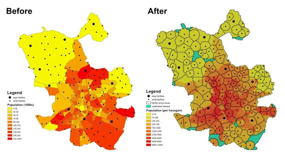
Die Planungsfrage ist einfach, aber nützlich: Gibt es angesichts der Bevölkerung in jedem Viertel oder Vorort, der Kapazität jeder Einrichtung und der maximalen Entfernung, die jede Einrichtung abdecken kann, genügend Einrichtungen, um die gesamte Bevölkerung zu versorgen, und wenn nicht, welche Gebiete bleiben unter den aktuellen Einschränkungen nicht zugewiesen?
Was das Modell macht
Dabei handelt es sich um ein Zuordnungs- und Standortzuordnungsmodell. Jeder Bedarfsstandort wird durch ein Sechseck dargestellt, jede Einrichtung stellt das verfügbare Angebot dar und das Modell weist jedes Sechseck einer einzelnen optimalen Einrichtung zu, wobei die Serviceentfernungs- und Kapazitätsregeln beachtet werden. Das gleiche Modellierungsmuster kann für Gesundheitseinrichtungen, Schulen, Banken, Einzelhandelsgeschäfte oder andere Servicenetzwerke verwendet werden, bei denen wir Abdeckung, Servicebereiche und Zugangslücken verstehen müssen.
Die Ausgabe ist nicht nur eine Tabelle mit Aufgaben. Es kann auch in Einzugsgebiets- und Handelsgebietsebenen umgewandelt werden, die zeigen, welche Standorte von jeder Einrichtung sinnvoll abgedeckt werden können, welche Bedarfsgebiete in einen nicht zugewiesenen Fallback verschoben werden und wie sich das Ergebnis ändert, wenn Kapazitäten, Entfernungen oder Ziele angepasst werden.
Zielfunktion
In diesem Beispiel besteht das Ziel darin, die Gesamtentfernung von jedem Nachfragesechseck zu der ihm zugewiesenen Einrichtung zu minimieren. Dies ergibt unter den aktuellen Annahmen die effizienteste Allokation. Dasselbe Framework kann mit einer anderen Zielfunktion erneut ausgeführt werden, wenn sich die Geschäftsfrage ändert. Beispielsweise können wir die Betriebskosten anstelle der Entfernung minimieren, die Reisezeit anstelle der Luftlinie minimieren oder die Nachfrage neu ausbalancieren, damit kostenintensivere Einrichtungen genug Volumen erhalten, um ihr Betriebsprofil zu rechtfertigen.
Wichtige Einschränkungen
- Jede Einrichtung hat eine maximale Serviceentfernung, daher kann ihr kein Bedarf außerhalb dieses Bereichs zugeordnet werden.
- Jede Anlage hat minimale und maximale Bevölkerungsgrenzen, daher muss der ihr zugewiesene Gesamtbedarf innerhalb ihrer Kapazitätsgrenzen bleiben.
- Jedes Nachfragesechseck muss einer einzelnen Einrichtung zugeordnet sein.
- Wenn ein Sechseck keiner realen Einrichtung zugeordnet werden kann, kann es einer Dummy-Einrichtung
unassignedzugewiesen werden, damit das Modell realisierbar bleibt und die Abdeckungslücke sichtbar ist. – Das Beispiel verwendet euklidische Abstände zwischen Sechseckschwerpunkten und Einrichtungen für schnelles Prototyping, aber der gleiche Arbeitsablauf kann bei Bedarf auf real befahrbare Routen umgestellt werden.
Arbeitsablauf
Der Workflow besteht aus drei Hauptphasen:
- Konvertieren Sie den interessierenden Bereich in eine sechseckige Tessellation und leiten Sie die Population für jedes Sechseck ab.
- Generieren Sie die Ursprungs-Ziel-Matrix zwischen jedem Nachfragesechseck und jeder Einrichtung.
- Lösen Sie das Optimierungsmodell und exportieren Sie die Ergebnisse nach GeoJSON, damit sie in QGIS, ArcGIS Pro oder einer anderen Kartierungssoftware überprüft werden können.
Der Implementierungsstapel umfasst Open-Source-Python mit Shapely-, Pyproj-, SQLite3-, Pyomo-, CBC-Solver- und GeoJSON-Ausgaben. Das Datenaufbereitungsmuster ist bewusst modular aufgebaut, was es einfach macht, die Nachfrageschicht zu ersetzen, die Anlagenbeschränkungen zu ändern, das Ziel auszutauschen oder das Modell um zusätzliche Geschäftsregeln zu erweitern.
Implementierungshinweise- PuLP wurde ursprünglich getestet, aber stattdessen wurde Pyomo ausgewählt, da es viel größere Modelle zuverlässiger verarbeiten konnte.
– Das Modell wurde mit dem Open-Source-CBC-Solver gelöst und dieser Ansatz konnte mit diesem Setup in weniger als einer Stunde auf mehr als 50 Millionen Entscheidungsvariablen skaliert werden.
- Für noch größere Instanzen kann Gurobi in Betracht gezogen werden, sofern die Lizenz dies zulässt. – Das Schreiben großer Ausgaben in GeoJSON kann länger dauern als das Lösen des Modells selbst. Daher kann es bei größeren Produktionsläufen effizienter sein, direkt in eine Datenbank zu schreiben. – Eine praktische Möglichkeit, solche Modelle zu erstellen, besteht darin, beim Testen von Einschränkungen mit großen Sechsecken und schnellen euklidischen Abständen zu beginnen und dann zu einer feineren Tessellation und realistischeren Routenkosten zu wechseln, sobald das Modellverhalten validiert ist.
- Zusätzliche Einschränkungen können schrittweise hinzugefügt werden, sollten jedoch sorgfältig eingeführt werden, da jede zusätzliche Geschäftsregel das Risiko erhöht, dass das Modell nicht mehr realisierbar ist.
Beispiel-Quellcode
Der folgende Code zeigt den End-to-End-Workflow direkt auf dieser Seite.
1. generic_hexagons.py
import json
import math
import os
import pyproj
from shapely.geometry import shape

# for converting the coordinates to and from geographic and projected coordinates
TRAN_4326_TO_3857 = pyproj.Transformer.from_crs("EPSG:4326", "EPSG:3857")
TRAN_3857_TO_4326 = pyproj.Transformer.from_crs("EPSG:3857", "EPSG:4326")

# the area of interest used for generating the hexagons
input_geojson_file = "input/area_of_interest.geojson"

# load the area of interest into a JSON object
with open(input_geojson_file) as json_file:
    geojson = json.load(json_file)

# the area of interest coordinates (note this is for a single-part / contiguous polygon)
geographic_coordinates = geojson["features"][0]["geometry"]["coordinates"]

# create an area of interest polygon using shapely
aoi = shape({"type": "Polygon", "coordinates": geographic_coordinates})

# get the geographic bounding box coordinates for the area of interest
(lng1, lat1, lng2, lat2) = aoi.bounds

# get the projected bounding box coordinates for the area of interest
[W, S] = TRAN_4326_TO_3857.transform(lat1, lng1)
[E, N] = TRAN_4326_TO_3857.transform(lat2, lng2)

# the area of interest height
aoi_height = N - S

# the area of interest width
aoi_width = E - W

# the length of the side of the hexagon
l = 200

# the length of the apothem of the hexagon
apo = l * math.sqrt(3) / 2

# distance from the mid-point of the hexagon side to the opposite side
d = 2 * apo

# the number of rows of hexagons
row_count = math.ceil(aoi_height / l / 1.5)

# add a row of hexagons if the hexagon tessallation does not fully cover the area of interest
if(row_count % 2 != 0 and row_count * l * 1.5 - l / 2 < aoi_height):
    row_count += 1

# the number of columns of hexagons
column_count = math.ceil(aoi_width / d) + 1

# the total height and width of the hexagons
total_height_of_hexagons = row_count * l * 1.5 if row_count % 2 == 0 else 1.5 * (row_count - 1) * l + l
total_width_of_hexagons = (column_count - 1) * d

# offsets to center the hexagon tessellation over the bounding box for the area of interest
x_offset = (total_width_of_hexagons - aoi_width) / 2
y_offset = (row_count * l * 3 / 2 - l / 2 - aoi_height - l) / 2

# create an empty feature collection for the hexagons
feature_collection = { "type": "FeatureCollection", "features": [] }

oid = 1

hexagon_count = 0

for i in range(0, column_count):
    for j in range(0, row_count):
        if(j % 2 == 0 or i < column_count - 1):
            x = W - x_offset + d * i if j % 2 == 0 else W - x_offset + apo + d * i
            y = S - y_offset + l * 1.5 * j

            coords = []

            for [lat, lng] in [
                TRAN_3857_TO_4326.transform(x, y + l),
                TRAN_3857_TO_4326.transform(x + apo, y + l / 2),
                TRAN_3857_TO_4326.transform(x + apo, y - l / 2),
                TRAN_3857_TO_4326.transform(x, y - l),
                TRAN_3857_TO_4326.transform(x - apo, y - l / 2),
                TRAN_3857_TO_4326.transform(x - apo, y + l / 2),
                TRAN_3857_TO_4326.transform(x, y + l)
            ]:
                coords.append([lng, lat])

            hexagon = shape({"type": "Polygon", "coordinates": [coords]})

            # check if the hexagon is within the area of interest
            if aoi.intersects(hexagon):
                hexagon_count += 1
                if(hexagon_count % 1000 == 0):
                    print('Generated {} hexagons'.format(hexagon_count))

                population = 0
                hexagon_names = []

                # open the geojson file with the population data
                with open("input/population_areas.geojson") as json_file:
                    geojson = json.load(json_file)

                    for feature in geojson["features"]:
                        polygon = shape(
                            {
                                "type": "Polygon",
                                "coordinates": feature["geometry"]["coordinates"]
                            }
                        )

                        # check if hexagon is within the polygon and derive the population for that intersected part of the hexagon
                        if hexagon.intersects(polygon):
                            if not feature["properties"]["Name"] in hexagon_names:
                                hexagon_names.append(feature["properties"]["Name"])

                            population += (
                                hexagon.intersection(polygon).area
                                / polygon.area
                                * feature["properties"]["Population"]
                            )

                hexagon_names.sort()

                f = {
                    "type": "Feature",
                    "properties": {
                        "id": oid,
                        "name": ', '.join(hexagon_names),
                        "population": population
                    },
                    "geometry": {
                            "type": "Polygon",
                            "coordinates": [coords]
                        }
                }

                # add the hexagon to the feature collection
                feature_collection['features'].append(f)

                oid += 1

print('Generated {} hexagons'.format(hexagon_count))

# output the feature collection to a geojson file
with open("output/hexagons.geojson", "w") as output_file:
    output_file.write(json.dumps(feature_collection))


# Play a sound when the script finishes (macOS)
for i in range(1, 2):
    os.system('afplay /System/Library/Sounds/Glass.aiff')

# Play a sound when the script finishes (Windows OS)
    # import time
    # import winsound

    # frequency = 1000
    # duration = 300

    # for i in range(1, 10):
    #     winsound.Beep(frequency, duration)
    #     time.sleep(0.1)
2. generic_origin_destination_matrix.py
import json
import math
import os
import pyproj
import sqlite3

def getDistance(x1,y1,x2,y2):
    distance = math.sqrt((x2-x1)**2+(y2-y1)**2)
    return int(distance)

def getHexagonCentroid(hexagon):
    coordinates = hexagon['geometry']['coordinates'][0]

    # remove the last pair of coordinates in the hexagon
    coordinates.pop()

    lat = sum(coords[1] for coords in coordinates) / 6
    lng = sum(coords[0] for coords in coordinates) / 6

    return lat, lng

# for converting the coordinates to and from geographic and projected coordinates
TRAN_4326_TO_3857 = pyproj.Transformer.from_crs("EPSG:4326", "EPSG:3857")
TRAN_3857_TO_4326 = pyproj.Transformer.from_crs("EPSG:3857", "EPSG:4326")

# create a sqlite database for the results
db = 'output/results.sqlite'

# delete the database if it already exists
if(os.path.exists(db)):
    os.remove(db)

# create a connection to the sqlite database
conn = sqlite3.connect(db)

# create cursors for the database connection
c1 = conn.cursor()
c2 = conn.cursor()

# create the facilities table
c1.execute('''
    CREATE TABLE facilities (
        facility_id                     INT,
        facility_x                      REAL,
        facility_y                      REAL,
        trade_area_distance_constraint  REAL,
        min_population_constraint       INT,
        max_population_constraint       INT
    );
''')

c1.execute('''
    CREATE TABLE od_matrix (
        facility_id INT,
        hexagon_id  INT,
        facility_x  REAL,
        facility_y  REAL,
        hexagon_x   REAL,
        hexagon_y   REAL,
        distance    INT,
        optimal     INT
    );
''')

# the geojson for the facilities
input_geojson_file = "input/facilities.geojson"

# load the area of interest into a JSON object
with open(input_geojson_file) as json_file:
    geojson = json.load(json_file)

    facilities = geojson['features']

    for facility in facilities:
        facility_id = facility['properties']['OID']
        trade_area_distance_constraint = facility['properties']['trade_area_dist_constraint']
        min_population_constraint = facility['properties']['min_population_constraint']
        max_population_constraint = facility['properties']['max_population_constraint']

        [lng, lat] = facility['geometry']['coordinates']
        [x, y] = TRAN_4326_TO_3857.transform(lat, lng)

        sql = '''
            INSERT INTO facilities (
                facility_id,
                facility_x,
                facility_y,
                trade_area_distance_constraint,
                min_population_constraint,
                max_population_constraint
            )
            VALUES ({},{},{},{},{},{});
        '''.format(facility_id, x, y, trade_area_distance_constraint, min_population_constraint, max_population_constraint)

        c1.execute(sql)

# create an empty feature collection for the hexagons
feature_collection = { "type": "FeatureCollection", "features": [] }

# the geojson for the hexagons
input_geojson_file = "output/hexagons.geojson"

# load the area of interest into a JSON object
with open(input_geojson_file) as json_file:
    geojson = json.load(json_file)

    hexagons = geojson['features']

    for i, hexagon in enumerate(hexagons):
        hexagon_id = hexagon['properties']['id']
        lat, lng = getHexagonCentroid(hexagon)
        [hexagon_x, hexagon_y] = TRAN_4326_TO_3857.transform(lat, lng)

        rows = c1.execute('''
            SELECT facility_id, facility_x, facility_y, trade_area_distance_constraint
            FROM facilities;
        ''').fetchall()

        for row in rows:
            facility_id, facility_x, facility_y, trade_area_distance_constraint = row
            distance = getDistance(hexagon_x, hexagon_y, facility_x, facility_y)

            if(distance > int(trade_area_distance_constraint)):
                distance = 100000

            sql = '''
                INSERT INTO od_matrix(facility_id, facility_x, facility_y, hexagon_id, hexagon_x, hexagon_y, distance)
                VALUES ({},{},{},{},{},{},{});
            '''.format(facility_id, facility_x, facility_y, hexagon_id, hexagon_x, hexagon_y, distance)

            c2.execute(sql)

            (hexagon_lat, hexagon_lng) = TRAN_3857_TO_4326.transform(hexagon_x, hexagon_y)
            (facility_lat, facility_lng) = TRAN_3857_TO_4326.transform(facility_x, facility_y)

            coords = [[facility_lng, facility_lat],[hexagon_lng, hexagon_lat]]

            if(distance <= trade_area_distance_constraint):
                f = {
                    "type": "Feature",
                    "properties": {},
                    "geometry": {
                            "type": "LineString",
                            "coordinates": coords
                        }
                }

                # add the hexagon to the feature collection
                feature_collection['features'].append(f)


        if((i+1) % 1000 == 0):
            print('Processed {} hexagons'.format(i+1))


conn.commit()
conn.close()

# output the feasible facility-hexagon pairs to geojson
with open("output/routes.geojson", "w") as output_file:
    output_file.write(json.dumps(feature_collection))

for i in range(1,2):
    os.system('afplay /System/Library/Sounds/Glass.aiff')
3.solve_the_model.py
from pyomo.environ import *
from pyomo.opt import SolverFactory
import datetime
import json
import os
import pyproj
import sqlite3

# for converting the coordinates to and from geographic and projected coordinates
TRAN_4326_TO_3857 = pyproj.Transformer.from_crs("EPSG:4326", "EPSG:3857")
TRAN_3857_TO_4326 = pyproj.Transformer.from_crs("EPSG:3857", "EPSG:4326")

# the input database created from the previous script
db = 'output/results.sqlite'

# create a database connection
conn = sqlite3.connect(db)

# create a cursor for the database connection
c = conn.cursor()

# the demand, supply, and cost matrices
Demand = {}
Supply = {}
Cost = {}

'''
    Supply['S0'] is for infeasible results, i.e. hexagons that do not
    have any facilities when the nearest facility is too far away,
    or when the population constraint for the facilities means the
    hexagon cannot be assigned to that facility
'''
# the population capacity constraint of the "unassigned" facility
Supply['S0'] = {}
Supply['S0']['min_pop'] = 0
Supply['S0']['max_pop'] = 1E10

sql = '''
    SELECT DISTINCT hexagon_id
    FROM od_matrix
    ORDER BY 1;
'''

# the assignment constraint, i.e. each hexagon can only be assigned to one facility
for row in c.execute(sql):
    hexagon_id = row[0]
    d = 'D{}'.format(hexagon_id)
    Demand[d] = 1

    # the infeasible case for each hexagon
    Cost[(d,'S0')] = 1E4

sql = '''
    SELECT DISTINCT facility_id, min_population_constraint, max_population_constraint
    FROM facilities
    ORDER BY 1;
'''

# the facility capacity constraint - cannot supply more hexagons than the facility has capacity for
for row in c.execute(sql):
    [facility_id, min_population_constraint, max_population_constraint] = row
    s = 'S{}'.format(facility_id)
    Supply[s] = {}
    Supply[s]['min_pop'] = min_population_constraint
    Supply[s]['max_pop'] = max_population_constraint

sql = '''
    SELECT facility_id, hexagon_id, distance
    FROM od_matrix;
'''

# creating the Cost matrix
for row in c.execute(sql):
    (facility_id, hexagon_id, distance) = row
    d = 'D{}'.format(hexagon_id)
    s = 'S{}'.format(facility_id)
    Cost[(d,s)] = distance

print('Building the model')

# creating the model
model = ConcreteModel()
model.dual = Suffix(direction=Suffix.IMPORT)

# Step 1: Define index sets
dem = list(Demand.keys())
sup = list(Supply.keys())

# Step 2: Define the decision variables
model.x = Var(dem, sup, domain=NonNegativeReals)

# Step 3: Define Objective
model.Cost = Objective(
    expr = sum([Cost[d,s]*model.x[d,s] for d in dem for s in sup]),
    sense = minimize
)

# Step 4: Constraints
model.sup = ConstraintList()
# each facility cannot supply more than its population capacity
for s in sup:
    model.sup.add(sum([model.x[d,s] for d in dem]) >= Supply[s]['min_pop'])
    model.sup.add(sum([model.x[d,s] for d in dem]) <= Supply[s]['max_pop'])

model.dmd = ConstraintList()
# each hexagon can only be assigned to one facility
for d in dem:
    model.dmd.add(sum([model.x[d,s] for s in sup]) == Demand[d])

'''
    There is no need to add a constraint for the service/trade area distances
    for the facilities. We are already handling this when we generate
    the origin destination matrix. If any hexagon falls outside of all
    facility trade areas, then it gets assigned to the "unassigned" facility.
'''

print('Solving the model')

# use the CBC solver and solve the model
results = SolverFactory('cbc').solve(model)

# for c in dem:
#     for s in sup:
#         print(c, s, model.x[c,s]())

# if the model solved correctly
if 'ok' == str(results.Solver.status):
    print("Objective Function = ", model.Cost())
    print('Outputting the results to GeoJSON') # note it would be faster to write the results directly to a database, e.g. Postgres / SQL Server

    # print("Results:")
    for s in sup:
        for d in dem:
            if model.x[d,s]() > 0:
                # print("From ", s," to ", d, ":", model.x[d,s]())
                facility_id = s.replace('S','')
                hexagon_id = d.replace('D','')
                c.execute('''
                    UPDATE od_matrix
                    SET optimal = 1
                    WHERE facility_id = {}
                        AND hexagon_id = {};
                '''.format(facility_id, hexagon_id))

    # create an empty feature collection for the results
    feature_collection = { "type": "FeatureCollection", "features": [] }

    rows = c.execute('''
            SELECT facility_id, hexagon_id, facility_x, facility_y, hexagon_x, hexagon_y, distance
            FROM od_matrix
            WHERE optimal = 1;
        ''')

    for row in rows:
        (facility_id, hexagon_id, facility_x, facility_y, hexagon_x, hexagon_y, distance) = row
        (hexagon_lat, hexagon_lng) = TRAN_3857_TO_4326.transform(hexagon_x, hexagon_y)
        (facility_lat, facility_lng) = TRAN_3857_TO_4326.transform(facility_x, facility_y)

        coords = [[facility_lng, facility_lat],[hexagon_lng, hexagon_lat]]

        f = {
                "type": "Feature",
                "properties": {},
                "geometry": {
                        "type": "LineString",
                        "coordinates": coords
                    }
            }

        # add the route to the feature collection
        feature_collection['features'].append(f)

    # output the optimally assigned pairs to geojson
    with open("output/optimal_results.geojson", "w") as output_file:
        output_file.write(json.dumps(feature_collection))

    # update the hexagons
    with open('output/hexagons.geojson') as json_file:
        geojson = json.load(json_file)
        hexagons = geojson['features']

        for hexagon in hexagons:
            facility_id = -1
            hexagon_id = hexagon['properties']['id']

            sql = '''
                SELECT facility_id
                FROM od_matrix
                WHERE hexagon_id = {}
                    AND optimal = 1;
            '''.format(hexagon_id)

            row = c.execute(sql).fetchone()

            if row:
                facility_id = row[0]

            hexagon['properties']['facility_id'] = facility_id

        # load the area of interest into a JSON object
        with open("output/hexagon_results.geojson", "w") as output_file:
            output_file.write(json.dumps(geojson))

else:
    print("No Feasible Solution Found")

finish_time = datetime.datetime.now()
# print('demand nodes = {} and supply nodes = {} | time = {}'.format(no_of_demand_nodes, no_of_supply_nodes, finish_time-start_time))

conn.commit()
conn.close()

for i in range(1,2):
    os.system('afplay /System/Library/Sounds/Glass.aiff')