Optimización de ubicación-asignación
Este ejemplo muestra cómo abordamos un problema grande de asignación y ubicación-asignación con Python de código abierto. El flujo utiliza datos anonimizados y demuestra cómo preparamos las entradas del modelo, construimos la matriz origen-destino, resolvimos la optimización y exportamos los resultados a GeoJSON para revisarlos en software SIG.
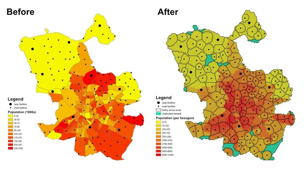
La pregunta de planificación es sencilla pero muy útil: dada la población de cada vecindario o suburbio, la capacidad de cada instalación y la distancia máxima que cada instalación puede atender, ¿existen suficientes instalaciones para atender a toda la población y, si no, qué zonas quedan sin asignar con las restricciones actuales?
Qué hace el modelo
Este es un modelo de asignación y ubicación-asignación. Cada ubicación de demanda se representa mediante un hexágono, cada instalación representa la oferta disponible y el modelo asigna cada hexágono a una única instalación óptima respetando las reglas de capacidad y distancia de servicio. El mismo patrón de modelado puede utilizarse para instalaciones sanitarias, escuelas, bancos, comercios u otras redes de servicios en las que necesitemos entender cobertura, áreas de servicio y brechas de acceso.
La salida no es solo una tabla de asignaciones. También puede convertirse en capas de áreas de servicio y áreas de influencia que muestran qué ubicaciones están cubiertas de forma factible por cada instalación, qué zonas de demanda terminan en un caso unassigned y cómo cambia el resultado cuando ajustamos capacidades, distancias u objetivos.
Función objetivo
En este ejemplo, la función objetivo consiste en minimizar la distancia total desde cada hexágono de demanda hasta la instalación asignada. Eso proporciona la asignación más eficiente bajo los supuestos actuales. El mismo marco puede volver a ejecutarse con otra función objetivo si cambia la pregunta de negocio. Por ejemplo, podemos minimizar coste operativo en lugar de distancia, minimizar tiempo de viaje en lugar de distancia en línea recta, o reequilibrar la demanda para que las instalaciones más costosas reciban suficiente volumen.
Restricciones clave
- Cada instalación tiene una distancia máxima de servicio, por lo que la demanda fuera de ese rango no puede asignarse a ella.
- Cada instalación tiene límites mínimos y máximos de población, por lo que la demanda total asignada debe mantenerse dentro de sus capacidades.
- Cada hexágono de demanda debe asignarse a una sola instalación.
- Si un hexágono no puede asignarse a ninguna instalación real, puede asignarse a una instalación ficticia
unassignedpara que el modelo siga siendo factible y la brecha de cobertura quede visible. - El ejemplo utiliza distancias euclidianas entre centroides de hexágonos e instalaciones para prototipado rápido, pero el mismo flujo puede cambiarse a rutas reales cuando sea necesario.
Flujo
El flujo tiene tres etapas principales:
- Convertir el área de interés en una teselación hexagonal y derivar la población para cada hexágono.
- Generar la matriz origen-destino entre cada hexágono de demanda y cada instalación.
- Resolver el modelo de optimización y exportar los resultados a GeoJSON para revisarlos en QGIS, ArcGIS Pro u otro software cartográfico.
La implementación utiliza Python de código abierto con shapely, pyproj, sqlite3, pyomo, el solver CBC y salidas en GeoJSON. El patrón de preparación de datos es deliberadamente modular, por lo que resulta sencillo sustituir la capa de demanda, cambiar las restricciones de las instalaciones, modificar la función objetivo o ampliar el modelo con reglas adicionales.
Notas de implementación
- Inicialmente se probó PuLP, pero finalmente se eligió pyomo porque manejaba modelos mucho más grandes con mayor fiabilidad.
- El modelo se resolvió con el solver de código abierto CBC, y con esta aproximación se pudieron resolver más de 50 millones de variables de decisión en menos de una hora con esa configuración.
- Para instancias todavía mayores, puede considerarse gurobi cuando la licencia lo permita.
- Escribir grandes salidas en GeoJSON puede tardar más que la propia resolución del modelo, por lo que en ejecuciones de producción más grandes puede ser más eficiente escribir directamente a una base de datos.
- Una forma práctica de construir modelos como este es comenzar con hexágonos grandes y distancias euclidianas rápidas mientras se prueban las restricciones, y después pasar a una teselación más fina y costes de ruta más realistas.
- Las restricciones adicionales pueden incorporarse de forma incremental, pero conviene hacerlo con cuidado porque cada nueva regla de negocio aumenta el riesgo de que el modelo se vuelva infactible.
Código fuente de ejemplo
El código siguiente se incluye para que el flujo completo pueda revisarse directamente en esta página.
1. generate_hexagons.py
import json
import math
import os
import pyproj
from shapely.geometry import shape

# for converting the coordinates to and from geographic and projected coordinates
TRAN_4326_TO_3857 = pyproj.Transformer.from_crs("EPSG:4326", "EPSG:3857")
TRAN_3857_TO_4326 = pyproj.Transformer.from_crs("EPSG:3857", "EPSG:4326")

# the area of interest used for generating the hexagons
input_geojson_file = "input/area_of_interest.geojson"

# load the area of interest into a JSON object
with open(input_geojson_file) as json_file:
    geojson = json.load(json_file)

# the area of interest coordinates (note this is for a single-part / contiguous polygon)
geographic_coordinates = geojson["features"][0]["geometry"]["coordinates"]

# create an area of interest polygon using shapely
aoi = shape({"type": "Polygon", "coordinates": geographic_coordinates})

# get the geographic bounding box coordinates for the area of interest
(lng1, lat1, lng2, lat2) = aoi.bounds

# get the projected bounding box coordinates for the area of interest
[W, S] = TRAN_4326_TO_3857.transform(lat1, lng1)
[E, N] = TRAN_4326_TO_3857.transform(lat2, lng2)

# the area of interest height
aoi_height = N - S

# the area of interest width
aoi_width = E - W

# the length of the side of the hexagon
l = 200

# the length of the apothem of the hexagon
apo = l * math.sqrt(3) / 2

# distance from the mid-point of the hexagon side to the opposite side
d = 2 * apo

# the number of rows of hexagons
row_count = math.ceil(aoi_height / l / 1.5)

# add a row of hexagons if the hexagon tessallation does not fully cover the area of interest
if(row_count % 2 != 0 and row_count * l * 1.5 - l / 2 < aoi_height):
    row_count += 1

# the number of columns of hexagons
column_count = math.ceil(aoi_width / d) + 1

# the total height and width of the hexagons
total_height_of_hexagons = row_count * l * 1.5 if row_count % 2 == 0 else 1.5 * (row_count - 1) * l + l
total_width_of_hexagons = (column_count - 1) * d

# offsets to center the hexagon tessellation over the bounding box for the area of interest
x_offset = (total_width_of_hexagons - aoi_width) / 2
y_offset = (row_count * l * 3 / 2 - l / 2 - aoi_height - l) / 2

# create an empty feature collection for the hexagons
feature_collection = { "type": "FeatureCollection", "features": [] }

oid = 1

hexagon_count = 0

for i in range(0, column_count):
    for j in range(0, row_count):
        if(j % 2 == 0 or i < column_count - 1):
            x = W - x_offset + d * i if j % 2 == 0 else W - x_offset + apo + d * i
            y = S - y_offset + l * 1.5 * j

            coords = []

            for [lat, lng] in [
                TRAN_3857_TO_4326.transform(x, y + l),
                TRAN_3857_TO_4326.transform(x + apo, y + l / 2),
                TRAN_3857_TO_4326.transform(x + apo, y - l / 2),
                TRAN_3857_TO_4326.transform(x, y - l),
                TRAN_3857_TO_4326.transform(x - apo, y - l / 2),
                TRAN_3857_TO_4326.transform(x - apo, y + l / 2),
                TRAN_3857_TO_4326.transform(x, y + l)
            ]:
                coords.append([lng, lat])

            hexagon = shape({"type": "Polygon", "coordinates": [coords]})

            # check if the hexagon is within the area of interest
            if aoi.intersects(hexagon):
                hexagon_count += 1
                if(hexagon_count % 1000 == 0):
                    print('Generated {} hexagons'.format(hexagon_count))

                population = 0
                hexagon_names = []

                # open the geojson file with the population data
                with open("input/population_areas.geojson") as json_file:
                    geojson = json.load(json_file)

                    for feature in geojson["features"]:
                        polygon = shape(
                            {
                                "type": "Polygon",
                                "coordinates": feature["geometry"]["coordinates"]
                            }
                        )

                        # check if hexagon is within the polygon and derive the population for that intersected part of the hexagon
                        if hexagon.intersects(polygon):
                            if not feature["properties"]["Name"] in hexagon_names:
                                hexagon_names.append(feature["properties"]["Name"])

                            population += (
                                hexagon.intersection(polygon).area
                                / polygon.area
                                * feature["properties"]["Population"]
                            )

                hexagon_names.sort()

                f = {
                    "type": "Feature",
                    "properties": {
                        "id": oid,
                        "name": ', '.join(hexagon_names),
                        "population": population
                    },
                    "geometry": {
                            "type": "Polygon",
                            "coordinates": [coords]
                        }
                }

                # add the hexagon to the feature collection
                feature_collection['features'].append(f)

                oid += 1

print('Generated {} hexagons'.format(hexagon_count))

# output the feature collection to a geojson file
with open("output/hexagons.geojson", "w") as output_file:
    output_file.write(json.dumps(feature_collection))


# Play a sound when the script finishes (macOS)
for i in range(1, 2):
    os.system('afplay /System/Library/Sounds/Glass.aiff')

# Play a sound when the script finishes (Windows OS)
    # import time
    # import winsound

    # frequency = 1000
    # duration = 300

    # for i in range(1, 10):
    #     winsound.Beep(frequency, duration)
    #     time.sleep(0.1)
2. generate_origin_destination_matrix.py
import json
import math
import os
import pyproj
import sqlite3

def getDistance(x1,y1,x2,y2):
    distance = math.sqrt((x2-x1)**2+(y2-y1)**2)
    return int(distance)

def getHexagonCentroid(hexagon):
    coordinates = hexagon['geometry']['coordinates'][0]

    # remove the last pair of coordinates in the hexagon
    coordinates.pop()

    lat = sum(coords[1] for coords in coordinates) / 6
    lng = sum(coords[0] for coords in coordinates) / 6

    return lat, lng

# for converting the coordinates to and from geographic and projected coordinates
TRAN_4326_TO_3857 = pyproj.Transformer.from_crs("EPSG:4326", "EPSG:3857")
TRAN_3857_TO_4326 = pyproj.Transformer.from_crs("EPSG:3857", "EPSG:4326")

# create a sqlite database for the results
db = 'output/results.sqlite'

# delete the database if it already exists
if(os.path.exists(db)):
    os.remove(db)

# create a connection to the sqlite database
conn = sqlite3.connect(db)

# create cursors for the database connection
c1 = conn.cursor()
c2 = conn.cursor()

# create the facilities table
c1.execute('''
    CREATE TABLE facilities (
        facility_id                     INT,
        facility_x                      REAL,
        facility_y                      REAL,
        trade_area_distance_constraint  REAL,
        min_population_constraint       INT,
        max_population_constraint       INT
    );
''')

c1.execute('''
    CREATE TABLE od_matrix (
        facility_id INT,
        hexagon_id  INT,
        facility_x  REAL,
        facility_y  REAL,
        hexagon_x   REAL,
        hexagon_y   REAL,
        distance    INT,
        optimal     INT
    );
''')

# the geojson for the facilities
input_geojson_file = "input/facilities.geojson"

# load the area of interest into a JSON object
with open(input_geojson_file) as json_file:
    geojson = json.load(json_file)

    facilities = geojson['features']

    for facility in facilities:
        facility_id = facility['properties']['OID']
        trade_area_distance_constraint = facility['properties']['trade_area_dist_constraint']
        min_population_constraint = facility['properties']['min_population_constraint']
        max_population_constraint = facility['properties']['max_population_constraint']

        [lng, lat] = facility['geometry']['coordinates']
        [x, y] = TRAN_4326_TO_3857.transform(lat, lng)

        sql = '''
            INSERT INTO facilities (
                facility_id,
                facility_x,
                facility_y,
                trade_area_distance_constraint,
                min_population_constraint,
                max_population_constraint
            )
            VALUES ({},{},{},{},{},{});
        '''.format(facility_id, x, y, trade_area_distance_constraint, min_population_constraint, max_population_constraint)

        c1.execute(sql)

# create an empty feature collection for the hexagons
feature_collection = { "type": "FeatureCollection", "features": [] }

# the geojson for the hexagons
input_geojson_file = "output/hexagons.geojson"

# load the area of interest into a JSON object
with open(input_geojson_file) as json_file:
    geojson = json.load(json_file)

    hexagons = geojson['features']

    for i, hexagon in enumerate(hexagons):
        hexagon_id = hexagon['properties']['id']
        lat, lng = getHexagonCentroid(hexagon)
        [hexagon_x, hexagon_y] = TRAN_4326_TO_3857.transform(lat, lng)

        rows = c1.execute('''
            SELECT facility_id, facility_x, facility_y, trade_area_distance_constraint
            FROM facilities;
        ''').fetchall()

        for row in rows:
            facility_id, facility_x, facility_y, trade_area_distance_constraint = row
            distance = getDistance(hexagon_x, hexagon_y, facility_x, facility_y)

            if(distance > int(trade_area_distance_constraint)):
                distance = 100000

            sql = '''
                INSERT INTO od_matrix(facility_id, facility_x, facility_y, hexagon_id, hexagon_x, hexagon_y, distance)
                VALUES ({},{},{},{},{},{},{});
            '''.format(facility_id, facility_x, facility_y, hexagon_id, hexagon_x, hexagon_y, distance)

            c2.execute(sql)

            (hexagon_lat, hexagon_lng) = TRAN_3857_TO_4326.transform(hexagon_x, hexagon_y)
            (facility_lat, facility_lng) = TRAN_3857_TO_4326.transform(facility_x, facility_y)

            coords = [[facility_lng, facility_lat],[hexagon_lng, hexagon_lat]]

            if(distance <= trade_area_distance_constraint):
                f = {
                    "type": "Feature",
                    "properties": {},
                    "geometry": {
                            "type": "LineString",
                            "coordinates": coords
                        }
                }

                # add the hexagon to the feature collection
                feature_collection['features'].append(f)


        if((i+1) % 1000 == 0):
            print('Processed {} hexagons'.format(i+1))


conn.commit()
conn.close()

# output the feasible facility-hexagon pairs to geojson
with open("output/routes.geojson", "w") as output_file:
    output_file.write(json.dumps(feature_collection))

for i in range(1,2):
    os.system('afplay /System/Library/Sounds/Glass.aiff')
3. solve_the_model.py
from pyomo.environ import *
from pyomo.opt import SolverFactory
import datetime
import json
import os
import pyproj
import sqlite3

# for converting the coordinates to and from geographic and projected coordinates
TRAN_4326_TO_3857 = pyproj.Transformer.from_crs("EPSG:4326", "EPSG:3857")
TRAN_3857_TO_4326 = pyproj.Transformer.from_crs("EPSG:3857", "EPSG:4326")

# the input database created from the previous script
db = 'output/results.sqlite'

# create a database connection
conn = sqlite3.connect(db)

# create a cursor for the database connection
c = conn.cursor()

# the demand, supply, and cost matrices
Demand = {}
Supply = {}
Cost = {}

'''
    Supply['S0'] is for infeasible results, i.e. hexagons that do not
    have any facilities when the nearest facility is too far away,
    or when the population constraint for the facilities means the
    hexagon cannot be assigned to that facility
'''
# the population capacity constraint of the "unassigned" facility
Supply['S0'] = {}
Supply['S0']['min_pop'] = 0
Supply['S0']['max_pop'] = 1E10

sql = '''
    SELECT DISTINCT hexagon_id
    FROM od_matrix
    ORDER BY 1;
'''

# the assignment constraint, i.e. each hexagon can only be assigned to one facility
for row in c.execute(sql):
    hexagon_id = row[0]
    d = 'D{}'.format(hexagon_id)
    Demand[d] = 1

    # the infeasible case for each hexagon
    Cost[(d,'S0')] = 1E4

sql = '''
    SELECT DISTINCT facility_id, min_population_constraint, max_population_constraint
    FROM facilities
    ORDER BY 1;
'''

# the facility capacity constraint - cannot supply more hexagons than the facility has capacity for
for row in c.execute(sql):
    [facility_id, min_population_constraint, max_population_constraint] = row
    s = 'S{}'.format(facility_id)
    Supply[s] = {}
    Supply[s]['min_pop'] = min_population_constraint
    Supply[s]['max_pop'] = max_population_constraint

sql = '''
    SELECT facility_id, hexagon_id, distance
    FROM od_matrix;
'''

# creating the Cost matrix
for row in c.execute(sql):
    (facility_id, hexagon_id, distance) = row
    d = 'D{}'.format(hexagon_id)
    s = 'S{}'.format(facility_id)
    Cost[(d,s)] = distance

print('Building the model')

# creating the model
model = ConcreteModel()
model.dual = Suffix(direction=Suffix.IMPORT)

# Step 1: Define index sets
dem = list(Demand.keys())
sup = list(Supply.keys())

# Step 2: Define the decision variables
model.x = Var(dem, sup, domain=NonNegativeReals)

# Step 3: Define Objective
model.Cost = Objective(
    expr = sum([Cost[d,s]*model.x[d,s] for d in dem for s in sup]),
    sense = minimize
)

# Step 4: Constraints
model.sup = ConstraintList()
# each facility cannot supply more than its population capacity
for s in sup:
    model.sup.add(sum([model.x[d,s] for d in dem]) >= Supply[s]['min_pop'])
    model.sup.add(sum([model.x[d,s] for d in dem]) <= Supply[s]['max_pop'])

model.dmd = ConstraintList()
# each hexagon can only be assigned to one facility
for d in dem:
    model.dmd.add(sum([model.x[d,s] for s in sup]) == Demand[d])

'''
    There is no need to add a constraint for the service/trade area distances
    for the facilities. We are already handling this when we generate
    the origin destination matrix. If any hexagon falls outside of all
    facility trade areas, then it gets assigned to the "unassigned" facility.
'''

print('Solving the model')

# use the CBC solver and solve the model
results = SolverFactory('cbc').solve(model)

# for c in dem:
#     for s in sup:
#         print(c, s, model.x[c,s]())

# if the model solved correctly
if 'ok' == str(results.Solver.status):
    print("Objective Function = ", model.Cost())
    print('Outputting the results to GeoJSON') # note it would be faster to write the results directly to a database, e.g. Postgres / SQL Server

    # print("Results:")
    for s in sup:
        for d in dem:
            if model.x[d,s]() > 0:
                # print("From ", s," to ", d, ":", model.x[d,s]())
                facility_id = s.replace('S','')
                hexagon_id = d.replace('D','')
                c.execute('''
                    UPDATE od_matrix
                    SET optimal = 1
                    WHERE facility_id = {}
                        AND hexagon_id = {};
                '''.format(facility_id, hexagon_id))

    # create an empty feature collection for the results
    feature_collection = { "type": "FeatureCollection", "features": [] }

    rows = c.execute('''
            SELECT facility_id, hexagon_id, facility_x, facility_y, hexagon_x, hexagon_y, distance
            FROM od_matrix
            WHERE optimal = 1;
        ''')

    for row in rows:
        (facility_id, hexagon_id, facility_x, facility_y, hexagon_x, hexagon_y, distance) = row
        (hexagon_lat, hexagon_lng) = TRAN_3857_TO_4326.transform(hexagon_x, hexagon_y)
        (facility_lat, facility_lng) = TRAN_3857_TO_4326.transform(facility_x, facility_y)

        coords = [[facility_lng, facility_lat],[hexagon_lng, hexagon_lat]]

        f = {
                "type": "Feature",
                "properties": {},
                "geometry": {
                        "type": "LineString",
                        "coordinates": coords
                    }
            }

        # add the route to the feature collection
        feature_collection['features'].append(f)

    # output the optimally assigned pairs to geojson
    with open("output/optimal_results.geojson", "w") as output_file:
        output_file.write(json.dumps(feature_collection))

    # update the hexagons
    with open('output/hexagons.geojson') as json_file:
        geojson = json.load(json_file)
        hexagons = geojson['features']

        for hexagon in hexagons:
            facility_id = -1
            hexagon_id = hexagon['properties']['id']

            sql = '''
                SELECT facility_id
                FROM od_matrix
                WHERE hexagon_id = {}
                    AND optimal = 1;
            '''.format(hexagon_id)

            row = c.execute(sql).fetchone()

            if row:
                facility_id = row[0]

            hexagon['properties']['facility_id'] = facility_id

        # load the area of interest into a JSON object
        with open("output/hexagon_results.geojson", "w") as output_file:
            output_file.write(json.dumps(geojson))

else:
    print("No Feasible Solution Found")

finish_time = datetime.datetime.now()
# print('demand nodes = {} and supply nodes = {} | time = {}'.format(no_of_demand_nodes, no_of_supply_nodes, finish_time-start_time))

conn.commit()
conn.close()

for i in range(1,2):
    os.system('afplay /System/Library/Sounds/Glass.aiff')