Otimização de alocação de localização
Este exemplo mostra como abordamos um grande problema de atribuição e alocação de localização usando Python de código aberto. O fluxo de trabalho utiliza dados anonimizados e demonstra como preparamos as entradas do modelo, construímos a matriz origem-destino, resolvemos a otimização e exportamos os resultados de volta para o GeoJSON para que possam ser revisados no software SIG.
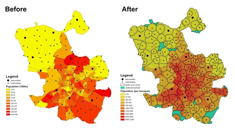
A questão do planeamento é simples mas útil: dada a população de cada bairro ou subúrbio, a capacidade de cada instalação e a distância máxima que cada instalação pode servir, existem instalações suficientes para servir toda a população e, se não, quais as áreas que permanecem não atribuídas sob as actuais restrições?
O que o modelo faz
Este é um modelo de atribuição e alocação de localização. Cada local de demanda é representado por um hexágono, cada instalação representa a oferta disponível e o modelo atribui cada hexágono a uma única instalação ideal, respeitando as regras de distância de serviço e capacidade. O mesmo padrão de modelação pode ser utilizado para instalações de saúde, escolas, bancos, lojas de retalho ou outras redes de serviços onde precisamos de compreender a cobertura, áreas de serviço e lacunas no acesso.
A saída não é apenas uma tabela de atribuições. Também pode ser transformado em camadas de área de serviço e de área comercial que mostram quais os locais que são viavelmente cobertos por cada instalação, quais as áreas de procura que são empurradas para um recurso não atribuído e como o resultado muda quando as capacidades, distâncias ou objectivos são ajustados.
Função objetivo
Para este exemplo, o objetivo é minimizar a distância total de cada hexágono de demanda até a instalação atribuída. Isso proporciona a alocação mais eficiente sob as atuais premissas. A mesma estrutura pode ser executada novamente com uma função objetivo diferente se a questão do negócio mudar. Por exemplo, podemos minimizar os custos operacionais em vez da distância, minimizar o tempo de viagem em vez da distância em linha reta ou reequilibrar a procura para que as instalações de custos mais elevados recebam volume suficiente para justificar o seu perfil operacional.
Principais restrições
- Cada instalação possui uma distância máxima de atendimento, portanto não poderá ser atribuída a ela demanda fora dessa faixa.
- Cada instalação tem limites mínimos e máximos de população, pelo que a procura total que lhe é atribuída deve permanecer dentro dos seus limites de capacidade.
- Cada hexágono de demanda deve ser atribuído a uma única instalação.
- Se um hexágono não puder ser atribuído a nenhuma instalação real, ele poderá ser alocado a uma instalação fictícia
unassignedpara que o modelo permaneça viável e a lacuna de cobertura seja visível. - O exemplo usa distâncias euclidianas entre centróides hexagonais e recursos para prototipagem rápida, mas o mesmo fluxo de trabalho pode ser alterado para rotas reais dirigíveis quando necessário.
Fluxo de trabalho
O fluxo de trabalho tem três etapas principais:
- Converta a área de interesse em um mosaico hexagonal e derive a população para cada hexágono.
- Gere a matriz origem-destino entre cada hexágono de demanda e cada instalação.
- Resolva o modelo de otimização e exporte os resultados para GeoJSON para que possam ser revisados no QGIS, ArcGIS Pro ou outro software de mapeamento.
A pilha de implementação inclui Python de código aberto com saídas shapely, pyproj, sqlite3, pyomo, o solucionador CBC e GeoJSON. O padrão de preparação de dados é deliberadamente modular, o que facilita a substituição da camada de demanda, a alteração das restrições das instalações, a troca do objetivo ou a extensão do modelo com regras de negócios adicionais.
Notas de implementação- O PuLP foi originalmente testado, mas o pyomo foi escolhido porque lidava com modelos muito maiores de maneira mais confiável.
- O modelo foi resolvido com o solucionador CBC de código aberto e essa abordagem foi dimensionada para mais de 50 milhões de variáveis de decisão em menos de uma hora com essa configuração.
- Para instâncias ainda maiores, o gurobi pode ser considerado onde o licenciamento permitir.
- Escrever grandes resultados no GeoJSON pode levar mais tempo do que resolver o modelo em si, portanto, para execuções de produção maiores, pode ser mais eficiente escrever diretamente em um banco de dados.
- Uma maneira prática de construir modelos como este é começar com hexágonos grandes e distâncias euclidianas rápidas enquanto testa as restrições, depois mudar para um mosaico mais fino e custos de rota mais realistas assim que o comportamento do modelo for validado.
- Restrições adicionais podem ser adicionadas de forma incremental, mas devem ser introduzidas com cuidado porque cada regra de negócio extra aumenta o risco de tornar o modelo inviável.
Exemplo de código fonte
O código abaixo mostra o fluxo de trabalho ponta a ponta diretamente nesta página.
1. generate_hexagons.py
import json
import math
import os
import pyproj
from shapely.geometry import shape

# for converting the coordinates to and from geographic and projected coordinates
TRAN_4326_TO_3857 = pyproj.Transformer.from_crs("EPSG:4326", "EPSG:3857")
TRAN_3857_TO_4326 = pyproj.Transformer.from_crs("EPSG:3857", "EPSG:4326")

# the area of interest used for generating the hexagons
input_geojson_file = "input/area_of_interest.geojson"

# load the area of interest into a JSON object
with open(input_geojson_file) as json_file:
    geojson = json.load(json_file)

# the area of interest coordinates (note this is for a single-part / contiguous polygon)
geographic_coordinates = geojson["features"][0]["geometry"]["coordinates"]

# create an area of interest polygon using shapely
aoi = shape({"type": "Polygon", "coordinates": geographic_coordinates})

# get the geographic bounding box coordinates for the area of interest
(lng1, lat1, lng2, lat2) = aoi.bounds

# get the projected bounding box coordinates for the area of interest
[W, S] = TRAN_4326_TO_3857.transform(lat1, lng1)
[E, N] = TRAN_4326_TO_3857.transform(lat2, lng2)

# the area of interest height
aoi_height = N - S

# the area of interest width
aoi_width = E - W

# the length of the side of the hexagon
l = 200

# the length of the apothem of the hexagon
apo = l * math.sqrt(3) / 2

# distance from the mid-point of the hexagon side to the opposite side
d = 2 * apo

# the number of rows of hexagons
row_count = math.ceil(aoi_height / l / 1.5)

# add a row of hexagons if the hexagon tessallation does not fully cover the area of interest
if(row_count % 2 != 0 and row_count * l * 1.5 - l / 2 < aoi_height):
    row_count += 1

# the number of columns of hexagons
column_count = math.ceil(aoi_width / d) + 1

# the total height and width of the hexagons
total_height_of_hexagons = row_count * l * 1.5 if row_count % 2 == 0 else 1.5 * (row_count - 1) * l + l
total_width_of_hexagons = (column_count - 1) * d

# offsets to center the hexagon tessellation over the bounding box for the area of interest
x_offset = (total_width_of_hexagons - aoi_width) / 2
y_offset = (row_count * l * 3 / 2 - l / 2 - aoi_height - l) / 2

# create an empty feature collection for the hexagons
feature_collection = { "type": "FeatureCollection", "features": [] }

oid = 1

hexagon_count = 0

for i in range(0, column_count):
    for j in range(0, row_count):
        if(j % 2 == 0 or i < column_count - 1):
            x = W - x_offset + d * i if j % 2 == 0 else W - x_offset + apo + d * i
            y = S - y_offset + l * 1.5 * j

            coords = []

            for [lat, lng] in [
                TRAN_3857_TO_4326.transform(x, y + l),
                TRAN_3857_TO_4326.transform(x + apo, y + l / 2),
                TRAN_3857_TO_4326.transform(x + apo, y - l / 2),
                TRAN_3857_TO_4326.transform(x, y - l),
                TRAN_3857_TO_4326.transform(x - apo, y - l / 2),
                TRAN_3857_TO_4326.transform(x - apo, y + l / 2),
                TRAN_3857_TO_4326.transform(x, y + l)
            ]:
                coords.append([lng, lat])

            hexagon = shape({"type": "Polygon", "coordinates": [coords]})

            # check if the hexagon is within the area of interest
            if aoi.intersects(hexagon):
                hexagon_count += 1
                if(hexagon_count % 1000 == 0):
                    print('Generated {} hexagons'.format(hexagon_count))

                population = 0
                hexagon_names = []

                # open the geojson file with the population data
                with open("input/population_areas.geojson") as json_file:
                    geojson = json.load(json_file)

                    for feature in geojson["features"]:
                        polygon = shape(
                            {
                                "type": "Polygon",
                                "coordinates": feature["geometry"]["coordinates"]
                            }
                        )

                        # check if hexagon is within the polygon and derive the population for that intersected part of the hexagon
                        if hexagon.intersects(polygon):
                            if not feature["properties"]["Name"] in hexagon_names:
                                hexagon_names.append(feature["properties"]["Name"])

                            population += (
                                hexagon.intersection(polygon).area
                                / polygon.area
                                * feature["properties"]["Population"]
                            )

                hexagon_names.sort()

                f = {
                    "type": "Feature",
                    "properties": {
                        "id": oid,
                        "name": ', '.join(hexagon_names),
                        "population": population
                    },
                    "geometry": {
                            "type": "Polygon",
                            "coordinates": [coords]
                        }
                }

                # add the hexagon to the feature collection
                feature_collection['features'].append(f)

                oid += 1

print('Generated {} hexagons'.format(hexagon_count))

# output the feature collection to a geojson file
with open("output/hexagons.geojson", "w") as output_file:
    output_file.write(json.dumps(feature_collection))


# Play a sound when the script finishes (macOS)
for i in range(1, 2):
    os.system('afplay /System/Library/Sounds/Glass.aiff')

# Play a sound when the script finishes (Windows OS)
    # import time
    # import winsound

    # frequency = 1000
    # duration = 300

    # for i in range(1, 10):
    #     winsound.Beep(frequency, duration)
    #     time.sleep(0.1)
2. generate_origin_destination_matrix.py
import json
import math
import os
import pyproj
import sqlite3

def getDistance(x1,y1,x2,y2):
    distance = math.sqrt((x2-x1)**2+(y2-y1)**2)
    return int(distance)

def getHexagonCentroid(hexagon):
    coordinates = hexagon['geometry']['coordinates'][0]

    # remove the last pair of coordinates in the hexagon
    coordinates.pop()

    lat = sum(coords[1] for coords in coordinates) / 6
    lng = sum(coords[0] for coords in coordinates) / 6

    return lat, lng

# for converting the coordinates to and from geographic and projected coordinates
TRAN_4326_TO_3857 = pyproj.Transformer.from_crs("EPSG:4326", "EPSG:3857")
TRAN_3857_TO_4326 = pyproj.Transformer.from_crs("EPSG:3857", "EPSG:4326")

# create a sqlite database for the results
db = 'output/results.sqlite'

# delete the database if it already exists
if(os.path.exists(db)):
    os.remove(db)

# create a connection to the sqlite database
conn = sqlite3.connect(db)

# create cursors for the database connection
c1 = conn.cursor()
c2 = conn.cursor()

# create the facilities table
c1.execute('''
    CREATE TABLE facilities (
        facility_id                     INT,
        facility_x                      REAL,
        facility_y                      REAL,
        trade_area_distance_constraint  REAL,
        min_population_constraint       INT,
        max_population_constraint       INT
    );
''')

c1.execute('''
    CREATE TABLE od_matrix (
        facility_id INT,
        hexagon_id  INT,
        facility_x  REAL,
        facility_y  REAL,
        hexagon_x   REAL,
        hexagon_y   REAL,
        distance    INT,
        optimal     INT
    );
''')

# the geojson for the facilities
input_geojson_file = "input/facilities.geojson"

# load the area of interest into a JSON object
with open(input_geojson_file) as json_file:
    geojson = json.load(json_file)

    facilities = geojson['features']

    for facility in facilities:
        facility_id = facility['properties']['OID']
        trade_area_distance_constraint = facility['properties']['trade_area_dist_constraint']
        min_population_constraint = facility['properties']['min_population_constraint']
        max_population_constraint = facility['properties']['max_population_constraint']

        [lng, lat] = facility['geometry']['coordinates']
        [x, y] = TRAN_4326_TO_3857.transform(lat, lng)

        sql = '''
            INSERT INTO facilities (
                facility_id,
                facility_x,
                facility_y,
                trade_area_distance_constraint,
                min_population_constraint,
                max_population_constraint
            )
            VALUES ({},{},{},{},{},{});
        '''.format(facility_id, x, y, trade_area_distance_constraint, min_population_constraint, max_population_constraint)

        c1.execute(sql)

# create an empty feature collection for the hexagons
feature_collection = { "type": "FeatureCollection", "features": [] }

# the geojson for the hexagons
input_geojson_file = "output/hexagons.geojson"

# load the area of interest into a JSON object
with open(input_geojson_file) as json_file:
    geojson = json.load(json_file)

    hexagons = geojson['features']

    for i, hexagon in enumerate(hexagons):
        hexagon_id = hexagon['properties']['id']
        lat, lng = getHexagonCentroid(hexagon)
        [hexagon_x, hexagon_y] = TRAN_4326_TO_3857.transform(lat, lng)

        rows = c1.execute('''
            SELECT facility_id, facility_x, facility_y, trade_area_distance_constraint
            FROM facilities;
        ''').fetchall()

        for row in rows:
            facility_id, facility_x, facility_y, trade_area_distance_constraint = row
            distance = getDistance(hexagon_x, hexagon_y, facility_x, facility_y)

            if(distance > int(trade_area_distance_constraint)):
                distance = 100000

            sql = '''
                INSERT INTO od_matrix(facility_id, facility_x, facility_y, hexagon_id, hexagon_x, hexagon_y, distance)
                VALUES ({},{},{},{},{},{},{});
            '''.format(facility_id, facility_x, facility_y, hexagon_id, hexagon_x, hexagon_y, distance)

            c2.execute(sql)

            (hexagon_lat, hexagon_lng) = TRAN_3857_TO_4326.transform(hexagon_x, hexagon_y)
            (facility_lat, facility_lng) = TRAN_3857_TO_4326.transform(facility_x, facility_y)

            coords = [[facility_lng, facility_lat],[hexagon_lng, hexagon_lat]]

            if(distance <= trade_area_distance_constraint):
                f = {
                    "type": "Feature",
                    "properties": {},
                    "geometry": {
                            "type": "LineString",
                            "coordinates": coords
                        }
                }

                # add the hexagon to the feature collection
                feature_collection['features'].append(f)


        if((i+1) % 1000 == 0):
            print('Processed {} hexagons'.format(i+1))


conn.commit()
conn.close()

# output the feasible facility-hexagon pairs to geojson
with open("output/routes.geojson", "w") as output_file:
    output_file.write(json.dumps(feature_collection))

for i in range(1,2):
    os.system('afplay /System/Library/Sounds/Glass.aiff')
3. resolver_o_modelo.py
from pyomo.environ import *
from pyomo.opt import SolverFactory
import datetime
import json
import os
import pyproj
import sqlite3

# for converting the coordinates to and from geographic and projected coordinates
TRAN_4326_TO_3857 = pyproj.Transformer.from_crs("EPSG:4326", "EPSG:3857")
TRAN_3857_TO_4326 = pyproj.Transformer.from_crs("EPSG:3857", "EPSG:4326")

# the input database created from the previous script
db = 'output/results.sqlite'

# create a database connection
conn = sqlite3.connect(db)

# create a cursor for the database connection
c = conn.cursor()

# the demand, supply, and cost matrices
Demand = {}
Supply = {}
Cost = {}

'''
    Supply['S0'] is for infeasible results, i.e. hexagons that do not
    have any facilities when the nearest facility is too far away,
    or when the population constraint for the facilities means the
    hexagon cannot be assigned to that facility
'''
# the population capacity constraint of the "unassigned" facility
Supply['S0'] = {}
Supply['S0']['min_pop'] = 0
Supply['S0']['max_pop'] = 1E10

sql = '''
    SELECT DISTINCT hexagon_id
    FROM od_matrix
    ORDER BY 1;
'''

# the assignment constraint, i.e. each hexagon can only be assigned to one facility
for row in c.execute(sql):
    hexagon_id = row[0]
    d = 'D{}'.format(hexagon_id)
    Demand[d] = 1

    # the infeasible case for each hexagon
    Cost[(d,'S0')] = 1E4

sql = '''
    SELECT DISTINCT facility_id, min_population_constraint, max_population_constraint
    FROM facilities
    ORDER BY 1;
'''

# the facility capacity constraint - cannot supply more hexagons than the facility has capacity for
for row in c.execute(sql):
    [facility_id, min_population_constraint, max_population_constraint] = row
    s = 'S{}'.format(facility_id)
    Supply[s] = {}
    Supply[s]['min_pop'] = min_population_constraint
    Supply[s]['max_pop'] = max_population_constraint

sql = '''
    SELECT facility_id, hexagon_id, distance
    FROM od_matrix;
'''

# creating the Cost matrix
for row in c.execute(sql):
    (facility_id, hexagon_id, distance) = row
    d = 'D{}'.format(hexagon_id)
    s = 'S{}'.format(facility_id)
    Cost[(d,s)] = distance

print('Building the model')

# creating the model
model = ConcreteModel()
model.dual = Suffix(direction=Suffix.IMPORT)

# Step 1: Define index sets
dem = list(Demand.keys())
sup = list(Supply.keys())

# Step 2: Define the decision variables
model.x = Var(dem, sup, domain=NonNegativeReals)

# Step 3: Define Objective
model.Cost = Objective(
    expr = sum([Cost[d,s]*model.x[d,s] for d in dem for s in sup]),
    sense = minimize
)

# Step 4: Constraints
model.sup = ConstraintList()
# each facility cannot supply more than its population capacity
for s in sup:
    model.sup.add(sum([model.x[d,s] for d in dem]) >= Supply[s]['min_pop'])
    model.sup.add(sum([model.x[d,s] for d in dem]) <= Supply[s]['max_pop'])

model.dmd = ConstraintList()
# each hexagon can only be assigned to one facility
for d in dem:
    model.dmd.add(sum([model.x[d,s] for s in sup]) == Demand[d])

'''
    There is no need to add a constraint for the service/trade area distances
    for the facilities. We are already handling this when we generate
    the origin destination matrix. If any hexagon falls outside of all
    facility trade areas, then it gets assigned to the "unassigned" facility.
'''

print('Solving the model')

# use the CBC solver and solve the model
results = SolverFactory('cbc').solve(model)

# for c in dem:
#     for s in sup:
#         print(c, s, model.x[c,s]())

# if the model solved correctly
if 'ok' == str(results.Solver.status):
    print("Objective Function = ", model.Cost())
    print('Outputting the results to GeoJSON') # note it would be faster to write the results directly to a database, e.g. Postgres / SQL Server

    # print("Results:")
    for s in sup:
        for d in dem:
            if model.x[d,s]() > 0:
                # print("From ", s," to ", d, ":", model.x[d,s]())
                facility_id = s.replace('S','')
                hexagon_id = d.replace('D','')
                c.execute('''
                    UPDATE od_matrix
                    SET optimal = 1
                    WHERE facility_id = {}
                        AND hexagon_id = {};
                '''.format(facility_id, hexagon_id))

    # create an empty feature collection for the results
    feature_collection = { "type": "FeatureCollection", "features": [] }

    rows = c.execute('''
            SELECT facility_id, hexagon_id, facility_x, facility_y, hexagon_x, hexagon_y, distance
            FROM od_matrix
            WHERE optimal = 1;
        ''')

    for row in rows:
        (facility_id, hexagon_id, facility_x, facility_y, hexagon_x, hexagon_y, distance) = row
        (hexagon_lat, hexagon_lng) = TRAN_3857_TO_4326.transform(hexagon_x, hexagon_y)
        (facility_lat, facility_lng) = TRAN_3857_TO_4326.transform(facility_x, facility_y)

        coords = [[facility_lng, facility_lat],[hexagon_lng, hexagon_lat]]

        f = {
                "type": "Feature",
                "properties": {},
                "geometry": {
                        "type": "LineString",
                        "coordinates": coords
                    }
            }

        # add the route to the feature collection
        feature_collection['features'].append(f)

    # output the optimally assigned pairs to geojson
    with open("output/optimal_results.geojson", "w") as output_file:
        output_file.write(json.dumps(feature_collection))

    # update the hexagons
    with open('output/hexagons.geojson') as json_file:
        geojson = json.load(json_file)
        hexagons = geojson['features']

        for hexagon in hexagons:
            facility_id = -1
            hexagon_id = hexagon['properties']['id']

            sql = '''
                SELECT facility_id
                FROM od_matrix
                WHERE hexagon_id = {}
                    AND optimal = 1;
            '''.format(hexagon_id)

            row = c.execute(sql).fetchone()

            if row:
                facility_id = row[0]

            hexagon['properties']['facility_id'] = facility_id

        # load the area of interest into a JSON object
        with open("output/hexagon_results.geojson", "w") as output_file:
            output_file.write(json.dumps(geojson))

else:
    print("No Feasible Solution Found")

finish_time = datetime.datetime.now()
# print('demand nodes = {} and supply nodes = {} | time = {}'.format(no_of_demand_nodes, no_of_supply_nodes, finish_time-start_time))

conn.commit()
conn.close()

for i in range(1,2):
    os.system('afplay /System/Library/Sounds/Glass.aiff')