Location-Allocation Optimisation
This example shows how we approach a large assignment and location-allocation problem using open-source Python. The workflow uses anonymised data and demonstrates how we prepare the model inputs, build the origin-destination matrix, solve the optimisation, and export the outputs back to GeoJSON so they can be reviewed in GIS software.
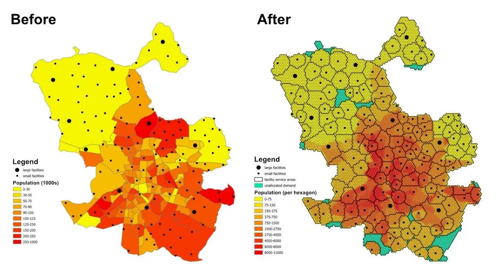
The planning question is simple but useful: given the population in each neighbourhood or suburb, the capacity of each facility, and the maximum distance each facility can serve, are there enough facilities to service the full population, and if not, which areas remain unassigned under the current constraints?
What the model does
This is an assignment and location-allocation model. Each demand location is represented by a hexagon, each facility represents available supply, and the model assigns every hexagon to a single optimal facility while respecting service-distance and capacity rules. The same modelling pattern can be used for healthcare facilities, schools, banks, retail stores, or other service networks where we need to understand coverage, service areas, and gaps in access.
The output is not just a table of assignments. It can also be turned into service-area and trade-area layers that show which locations are feasibly covered by each facility, which demand areas are pushed to an unassigned fallback, and how the result changes when capacities, distances, or objectives are adjusted.
Objective function
For this example, the objective is to minimise the total distance from every demand hexagon to its assigned facility. That gives the most efficient allocation under the current assumptions. The same framework can be rerun with a different objective function if the business question changes. For example, we can minimise operating cost instead of distance, minimise travel time instead of straight-line distance, or rebalance demand so higher-cost facilities receive enough volume to justify their operating profile.
Key constraints
- Each facility has a maximum service distance, so demand outside that range cannot be assigned to it.
- Each facility has minimum and maximum population bounds, so the total demand assigned to it must stay within its capacity limits.
- Each demand hexagon must be assigned to a single facility.
- If a hexagon cannot be assigned to any real facility, it can be allocated to a dummy
unassignedfacility so the model stays feasible and the coverage gap is visible. - The example uses Euclidean distances between hexagon centroids and facilities for fast prototyping, but the same workflow can be switched to real drivable routes when needed.
Workflow
The workflow has three main stages:
- Convert the area of interest into a hexagonal tessellation and derive the population for each hexagon.
- Generate the origin-destination matrix between each demand hexagon and each facility.
- Solve the optimisation model and export the results to GeoJSON so they can be reviewed in QGIS, ArcGIS Pro, or other mapping software.
The implementation stack includes open-source Python with shapely, pyproj, sqlite3, pyomo, the CBC solver, and GeoJSON outputs. The data-preparation pattern is deliberately modular, which makes it easy to replace the demand layer, change the facility constraints, swap out the objective, or extend the model with additional business rules.
Implementation notes
- PuLP was originally tested, but pyomo was chosen instead because it handled much larger models more reliably.
- The model was solved with the open-source CBC solver, and this approach scaled to more than 50 million decision variables in less than an hour with that setup.
- For even larger instances, gurobi can be considered where licensing allows it.
- Writing large outputs to GeoJSON can take longer than solving the model itself, so for bigger production runs it can be more efficient to write directly to a database.
- A practical way to build models like this is to start with large hexagons and fast Euclidean distances while testing constraints, then switch to finer tessellation and more realistic route costs once the model behaviour is validated.
- Additional constraints can be added incrementally, but they should be introduced carefully because each extra business rule increases the risk of making the model infeasible.
Example source code
The code below shows the end-to-end workflow directly on this page.
1. generate_hexagons.py
import json
import math
import os
import pyproj
from shapely.geometry import shape

# for converting the coordinates to and from geographic and projected coordinates
TRAN_4326_TO_3857 = pyproj.Transformer.from_crs("EPSG:4326", "EPSG:3857")
TRAN_3857_TO_4326 = pyproj.Transformer.from_crs("EPSG:3857", "EPSG:4326")

# the area of interest used for generating the hexagons
input_geojson_file = "input/area_of_interest.geojson"

# load the area of interest into a JSON object
with open(input_geojson_file) as json_file:
    geojson = json.load(json_file)

# the area of interest coordinates (note this is for a single-part / contiguous polygon)
geographic_coordinates = geojson["features"][0]["geometry"]["coordinates"]

# create an area of interest polygon using shapely
aoi = shape({"type": "Polygon", "coordinates": geographic_coordinates})

# get the geographic bounding box coordinates for the area of interest
(lng1, lat1, lng2, lat2) = aoi.bounds

# get the projected bounding box coordinates for the area of interest
[W, S] = TRAN_4326_TO_3857.transform(lat1, lng1)
[E, N] = TRAN_4326_TO_3857.transform(lat2, lng2)

# the area of interest height
aoi_height = N - S

# the area of interest width
aoi_width = E - W

# the length of the side of the hexagon
l = 200

# the length of the apothem of the hexagon
apo = l * math.sqrt(3) / 2

# distance from the mid-point of the hexagon side to the opposite side
d = 2 * apo

# the number of rows of hexagons
row_count = math.ceil(aoi_height / l / 1.5)

# add a row of hexagons if the hexagon tessallation does not fully cover the area of interest
if(row_count % 2 != 0 and row_count * l * 1.5 - l / 2 < aoi_height):
    row_count += 1

# the number of columns of hexagons
column_count = math.ceil(aoi_width / d) + 1

# the total height and width of the hexagons
total_height_of_hexagons = row_count * l * 1.5 if row_count % 2 == 0 else 1.5 * (row_count - 1) * l + l
total_width_of_hexagons = (column_count - 1) * d

# offsets to center the hexagon tessellation over the bounding box for the area of interest
x_offset = (total_width_of_hexagons - aoi_width) / 2
y_offset = (row_count * l * 3 / 2 - l / 2 - aoi_height - l) / 2

# create an empty feature collection for the hexagons
feature_collection = { "type": "FeatureCollection", "features": [] }

oid = 1

hexagon_count = 0

for i in range(0, column_count):
    for j in range(0, row_count):
        if(j % 2 == 0 or i < column_count - 1):
            x = W - x_offset + d * i if j % 2 == 0 else W - x_offset + apo + d * i
            y = S - y_offset + l * 1.5 * j

            coords = []

            for [lat, lng] in [
                TRAN_3857_TO_4326.transform(x, y + l),
                TRAN_3857_TO_4326.transform(x + apo, y + l / 2),
                TRAN_3857_TO_4326.transform(x + apo, y - l / 2),
                TRAN_3857_TO_4326.transform(x, y - l),
                TRAN_3857_TO_4326.transform(x - apo, y - l / 2),
                TRAN_3857_TO_4326.transform(x - apo, y + l / 2),
                TRAN_3857_TO_4326.transform(x, y + l)
            ]:
                coords.append([lng, lat])

            hexagon = shape({"type": "Polygon", "coordinates": [coords]})

            # check if the hexagon is within the area of interest
            if aoi.intersects(hexagon):
                hexagon_count += 1
                if(hexagon_count % 1000 == 0):
                    print('Generated {} hexagons'.format(hexagon_count))

                population = 0
                hexagon_names = []

                # open the geojson file with the population data
                with open("input/population_areas.geojson") as json_file:
                    geojson = json.load(json_file)

                    for feature in geojson["features"]:
                        polygon = shape(
                            {
                                "type": "Polygon",
                                "coordinates": feature["geometry"]["coordinates"]
                            }
                        )

                        # check if hexagon is within the polygon and derive the population for that intersected part of the hexagon
                        if hexagon.intersects(polygon):
                            if not feature["properties"]["Name"] in hexagon_names:
                                hexagon_names.append(feature["properties"]["Name"])

                            population += (
                                hexagon.intersection(polygon).area
                                / polygon.area
                                * feature["properties"]["Population"]
                            )

                hexagon_names.sort()

                f = {
                    "type": "Feature",
                    "properties": {
                        "id": oid,
                        "name": ', '.join(hexagon_names),
                        "population": population
                    },
                    "geometry": {
                            "type": "Polygon",
                            "coordinates": [coords]
                        }
                }

                # add the hexagon to the feature collection
                feature_collection['features'].append(f)

                oid += 1

print('Generated {} hexagons'.format(hexagon_count))

# output the feature collection to a geojson file
with open("output/hexagons.geojson", "w") as output_file:
    output_file.write(json.dumps(feature_collection))


# Play a sound when the script finishes (macOS)
for i in range(1, 2):
    os.system('afplay /System/Library/Sounds/Glass.aiff')

# Play a sound when the script finishes (Windows OS)
    # import time
    # import winsound

    # frequency = 1000
    # duration = 300

    # for i in range(1, 10):
    #     winsound.Beep(frequency, duration)
    #     time.sleep(0.1)
2. generate_origin_destination_matrix.py
import json
import math
import os
import pyproj
import sqlite3

def getDistance(x1,y1,x2,y2):
    distance = math.sqrt((x2-x1)**2+(y2-y1)**2)
    return int(distance)

def getHexagonCentroid(hexagon):
    coordinates = hexagon['geometry']['coordinates'][0]

    # remove the last pair of coordinates in the hexagon
    coordinates.pop()

    lat = sum(coords[1] for coords in coordinates) / 6
    lng = sum(coords[0] for coords in coordinates) / 6

    return lat, lng

# for converting the coordinates to and from geographic and projected coordinates
TRAN_4326_TO_3857 = pyproj.Transformer.from_crs("EPSG:4326", "EPSG:3857")
TRAN_3857_TO_4326 = pyproj.Transformer.from_crs("EPSG:3857", "EPSG:4326")

# create a sqlite database for the results
db = 'output/results.sqlite'

# delete the database if it already exists
if(os.path.exists(db)):
    os.remove(db)

# create a connection to the sqlite database
conn = sqlite3.connect(db)

# create cursors for the database connection
c1 = conn.cursor()
c2 = conn.cursor()

# create the facilities table
c1.execute('''
    CREATE TABLE facilities (
        facility_id                     INT,
        facility_x                      REAL,
        facility_y                      REAL,
        trade_area_distance_constraint  REAL,
        min_population_constraint       INT,
        max_population_constraint       INT
    );
''')

c1.execute('''
    CREATE TABLE od_matrix (
        facility_id INT,
        hexagon_id  INT,
        facility_x  REAL,
        facility_y  REAL,
        hexagon_x   REAL,
        hexagon_y   REAL,
        distance    INT,
        optimal     INT
    );
''')

# the geojson for the facilities
input_geojson_file = "input/facilities.geojson"

# load the area of interest into a JSON object
with open(input_geojson_file) as json_file:
    geojson = json.load(json_file)

    facilities = geojson['features']

    for facility in facilities:
        facility_id = facility['properties']['OID']
        trade_area_distance_constraint = facility['properties']['trade_area_dist_constraint']
        min_population_constraint = facility['properties']['min_population_constraint']
        max_population_constraint = facility['properties']['max_population_constraint']

        [lng, lat] = facility['geometry']['coordinates']
        [x, y] = TRAN_4326_TO_3857.transform(lat, lng)

        sql = '''
            INSERT INTO facilities (
                facility_id,
                facility_x,
                facility_y,
                trade_area_distance_constraint,
                min_population_constraint,
                max_population_constraint
            )
            VALUES ({},{},{},{},{},{});
        '''.format(facility_id, x, y, trade_area_distance_constraint, min_population_constraint, max_population_constraint)

        c1.execute(sql)

# create an empty feature collection for the hexagons
feature_collection = { "type": "FeatureCollection", "features": [] }

# the geojson for the hexagons
input_geojson_file = "output/hexagons.geojson"

# load the area of interest into a JSON object
with open(input_geojson_file) as json_file:
    geojson = json.load(json_file)

    hexagons = geojson['features']

    for i, hexagon in enumerate(hexagons):
        hexagon_id = hexagon['properties']['id']
        lat, lng = getHexagonCentroid(hexagon)
        [hexagon_x, hexagon_y] = TRAN_4326_TO_3857.transform(lat, lng)

        rows = c1.execute('''
            SELECT facility_id, facility_x, facility_y, trade_area_distance_constraint
            FROM facilities;
        ''').fetchall()

        for row in rows:
            facility_id, facility_x, facility_y, trade_area_distance_constraint = row
            distance = getDistance(hexagon_x, hexagon_y, facility_x, facility_y)

            if(distance > int(trade_area_distance_constraint)):
                distance = 100000

            sql = '''
                INSERT INTO od_matrix(facility_id, facility_x, facility_y, hexagon_id, hexagon_x, hexagon_y, distance)
                VALUES ({},{},{},{},{},{},{});
            '''.format(facility_id, facility_x, facility_y, hexagon_id, hexagon_x, hexagon_y, distance)

            c2.execute(sql)

            (hexagon_lat, hexagon_lng) = TRAN_3857_TO_4326.transform(hexagon_x, hexagon_y)
            (facility_lat, facility_lng) = TRAN_3857_TO_4326.transform(facility_x, facility_y)

            coords = [[facility_lng, facility_lat],[hexagon_lng, hexagon_lat]]

            if(distance <= trade_area_distance_constraint):
                f = {
                    "type": "Feature",
                    "properties": {},
                    "geometry": {
                            "type": "LineString",
                            "coordinates": coords
                        }
                }

                # add the hexagon to the feature collection
                feature_collection['features'].append(f)


        if((i+1) % 1000 == 0):
            print('Processed {} hexagons'.format(i+1))


conn.commit()
conn.close()

# output the feasible facility-hexagon pairs to geojson
with open("output/routes.geojson", "w") as output_file:
    output_file.write(json.dumps(feature_collection))

for i in range(1,2):
    os.system('afplay /System/Library/Sounds/Glass.aiff')
3. solve_the_model.py
from pyomo.environ import *
from pyomo.opt import SolverFactory
import datetime
import json
import os
import pyproj
import sqlite3

# for converting the coordinates to and from geographic and projected coordinates
TRAN_4326_TO_3857 = pyproj.Transformer.from_crs("EPSG:4326", "EPSG:3857")
TRAN_3857_TO_4326 = pyproj.Transformer.from_crs("EPSG:3857", "EPSG:4326")

# the input database created from the previous script
db = 'output/results.sqlite'

# create a database connection
conn = sqlite3.connect(db)

# create a cursor for the database connection
c = conn.cursor()

# the demand, supply, and cost matrices
Demand = {}
Supply = {}
Cost = {}

'''
    Supply['S0'] is for infeasible results, i.e. hexagons that do not
    have any facilities when the nearest facility is too far away,
    or when the population constraint for the facilities means the
    hexagon cannot be assigned to that facility
'''
# the population capacity constraint of the "unassigned" facility
Supply['S0'] = {}
Supply['S0']['min_pop'] = 0
Supply['S0']['max_pop'] = 1E10

sql = '''
    SELECT DISTINCT hexagon_id
    FROM od_matrix
    ORDER BY 1;
'''

# the assignment constraint, i.e. each hexagon can only be assigned to one facility
for row in c.execute(sql):
    hexagon_id = row[0]
    d = 'D{}'.format(hexagon_id)
    Demand[d] = 1

    # the infeasible case for each hexagon
    Cost[(d,'S0')] = 1E4

sql = '''
    SELECT DISTINCT facility_id, min_population_constraint, max_population_constraint
    FROM facilities
    ORDER BY 1;
'''

# the facility capacity constraint - cannot supply more hexagons than the facility has capacity for
for row in c.execute(sql):
    [facility_id, min_population_constraint, max_population_constraint] = row
    s = 'S{}'.format(facility_id)
    Supply[s] = {}
    Supply[s]['min_pop'] = min_population_constraint
    Supply[s]['max_pop'] = max_population_constraint

sql = '''
    SELECT facility_id, hexagon_id, distance
    FROM od_matrix;
'''

# creating the Cost matrix
for row in c.execute(sql):
    (facility_id, hexagon_id, distance) = row
    d = 'D{}'.format(hexagon_id)
    s = 'S{}'.format(facility_id)
    Cost[(d,s)] = distance

print('Building the model')

# creating the model
model = ConcreteModel()
model.dual = Suffix(direction=Suffix.IMPORT)

# Step 1: Define index sets
dem = list(Demand.keys())
sup = list(Supply.keys())

# Step 2: Define the decision variables
model.x = Var(dem, sup, domain=NonNegativeReals)

# Step 3: Define Objective
model.Cost = Objective(
    expr = sum([Cost[d,s]*model.x[d,s] for d in dem for s in sup]),
    sense = minimize
)

# Step 4: Constraints
model.sup = ConstraintList()
# each facility cannot supply more than its population capacity
for s in sup:
    model.sup.add(sum([model.x[d,s] for d in dem]) >= Supply[s]['min_pop'])
    model.sup.add(sum([model.x[d,s] for d in dem]) <= Supply[s]['max_pop'])

model.dmd = ConstraintList()
# each hexagon can only be assigned to one facility
for d in dem:
    model.dmd.add(sum([model.x[d,s] for s in sup]) == Demand[d])

'''
    There is no need to add a constraint for the service/trade area distances
    for the facilities. We are already handling this when we generate
    the origin destination matrix. If any hexagon falls outside of all
    facility trade areas, then it gets assigned to the "unassigned" facility.
'''

print('Solving the model')

# use the CBC solver and solve the model
results = SolverFactory('cbc').solve(model)

# for c in dem:
#     for s in sup:
#         print(c, s, model.x[c,s]())

# if the model solved correctly
if 'ok' == str(results.Solver.status):
    print("Objective Function = ", model.Cost())
    print('Outputting the results to GeoJSON') # note it would be faster to write the results directly to a database, e.g. Postgres / SQL Server

    # print("Results:")
    for s in sup:
        for d in dem:
            if model.x[d,s]() > 0:
                # print("From ", s," to ", d, ":", model.x[d,s]())
                facility_id = s.replace('S','')
                hexagon_id = d.replace('D','')
                c.execute('''
                    UPDATE od_matrix
                    SET optimal = 1
                    WHERE facility_id = {}
                        AND hexagon_id = {};
                '''.format(facility_id, hexagon_id))

    # create an empty feature collection for the results
    feature_collection = { "type": "FeatureCollection", "features": [] }

    rows = c.execute('''
            SELECT facility_id, hexagon_id, facility_x, facility_y, hexagon_x, hexagon_y, distance
            FROM od_matrix
            WHERE optimal = 1;
        ''')

    for row in rows:
        (facility_id, hexagon_id, facility_x, facility_y, hexagon_x, hexagon_y, distance) = row
        (hexagon_lat, hexagon_lng) = TRAN_3857_TO_4326.transform(hexagon_x, hexagon_y)
        (facility_lat, facility_lng) = TRAN_3857_TO_4326.transform(facility_x, facility_y)

        coords = [[facility_lng, facility_lat],[hexagon_lng, hexagon_lat]]

        f = {
                "type": "Feature",
                "properties": {},
                "geometry": {
                        "type": "LineString",
                        "coordinates": coords
                    }
            }

        # add the route to the feature collection
        feature_collection['features'].append(f)

    # output the optimally assigned pairs to geojson
    with open("output/optimal_results.geojson", "w") as output_file:
        output_file.write(json.dumps(feature_collection))

    # update the hexagons
    with open('output/hexagons.geojson') as json_file:
        geojson = json.load(json_file)
        hexagons = geojson['features']

        for hexagon in hexagons:
            facility_id = -1
            hexagon_id = hexagon['properties']['id']

            sql = '''
                SELECT facility_id
                FROM od_matrix
                WHERE hexagon_id = {}
                    AND optimal = 1;
            '''.format(hexagon_id)

            row = c.execute(sql).fetchone()

            if row:
                facility_id = row[0]

            hexagon['properties']['facility_id'] = facility_id

        # load the area of interest into a JSON object
        with open("output/hexagon_results.geojson", "w") as output_file:
            output_file.write(json.dumps(geojson))

else:
    print("No Feasible Solution Found")

finish_time = datetime.datetime.now()
# print('demand nodes = {} and supply nodes = {} | time = {}'.format(no_of_demand_nodes, no_of_supply_nodes, finish_time-start_time))

conn.commit()
conn.close()

for i in range(1,2):
    os.system('afplay /System/Library/Sounds/Glass.aiff')